Acquiring data with the Beaglehole Picometer Ellipsometer


This is an extremely flexible and powerful instrument; the method described below is what is required only for the simplest measurements. For more demanding applications either consult the manual or email the SAF.

First open Igor Pro, then open the PicoElli Control Panel in the bi menu. This panel is used to configure and take the measurement it is split into 10 parts 9 are shown below; the tenth is the monochromator control section:

Click on a part to find out more about what each input does. Make sure all the parameters are correct before you click the Measure button to acquire data. To find out about exporting and modeling the data click here.


Optical Table Control
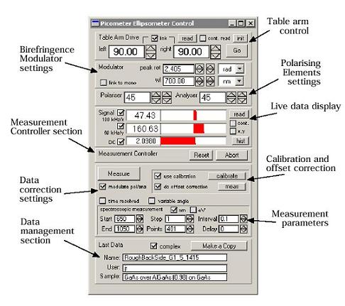
The main controls in the table arm drive section are the position input fields for the left and right arm. To drive the table, enter the desired positions into these fields and click the ‘Go’ button.
The input fields can be linked together with the ‘link’ checkbox that is located above the fields. When linked, if a value is entered into any of the two fields, it will be copied into the other field automatically.
The input fields also double as displays when reading the current arm position. Click the ‘read’ button for a single readout of both arm positions, or check the ‘cont. read’ box for a continuous readout. Continuous readout is stopped automatically when a value is entered into one of the position input fields.
The Optical Table has absolute angle encoders which allow absolute positioning of the arms with high accuracy. The ‘init’ button is used to initialise the arm drive’s position tracking. In order for the Measurement Controller to know the actual arm position, it first has to drive the arm to a reference position, also called end stop. After the table drive has been powered up, an initialisation must be carried out to re-establish the reference. When ‘init’ is clicked, a dialog box prompts for the approximate current position of the arms. Read the positions off the markings on the table enter and click OK. The arm positions are tracked continuously, and hence after this initialisation has been performed for the first time the position tracking remains active, even if the Optical Table Drive is switched off at the front panel. There is no need to re-initialise unless all power to the drive unit is lost completely.
.


Monochromator Control
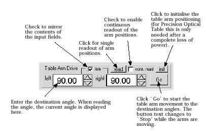
This section is only available when the instrument is configured for spectroscopic measurements. The monochromator’s wavelength position can be entered in nm or as photon energy in eV. The monochromator is driven to the selected position when the ‘Go’ button is clicked. The ‘init’ button is used to initialise the monochromator this re-establishes communications if they were lost, or if the monochromator was not on when the Controller was started. The ‘set’ button has no effect.


Birefringence Modulator Control
.
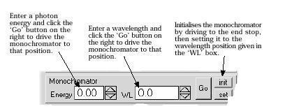
The Birefringence Modulator is controlled through a voltage from the Measurement Controller. Spectroscopic calibration data is stored on the Controller which it uses to calculate the Modulator gauge voltage for a given wavelength and peak retardance amplitude (or phase shift) setting. The Birefringence Modulator Section of the Picometer Ellipsometer Control panel allows you to set the Modulator retardation for a given wavelength and peak retardance amplitude, or by specifying the control voltage directly. This is done through the two input fields whose options can be set using popup menus (Variables: peak ret – peak phaseshift and wl – wavelength. Units: rad – radians, frac – fraction of the wavelength, volt – control voltage, nm – nanometers and eV – electron volts).
The value for the peak phaseshift for the single wavelength configuration of the Picometer Ellipsometer should be 2.405 rad. In a spectroscopic system, the Controller’s modulator calibration is used to set the modulator to the specified peak retardation at a given wave-length. If the ‘link to mono’ box is checked, the automatically modulator follows the monochromator’s wavelength setting so that the peak phaseshift stays constant across the spectral range.


Polariser and Analyser Control

This section is used to set the angular positions of polariser and analyser. After system startup, the rotating mounts must be initialised. In the Picometer Ellipsometer Control panel, this is done with the
‘Reset’ button in the Measurement Controller section of the panel.
For ellipsometry measurements, both the polariser and the analyser should be set to 45o. However, under certain conditions it may be desirable to set the analyser to other angles. When a measurement is started, the current position of the analyser will be used. If analyzer modulation is selected, the modulation is always symmetric within the four quadrants of the modulation, even if the angle is not 45o.
The settings in the input fields in the polariser and analyser section do not always represent the true positions of the rotating mounts. For example, in a measurement with modulated analyser, to save time the analyser is not automatically returned to its original position. Therefore its position may be 90o off when the measurement is finished. To make sure that the settings in the control panel are the real positions of the polarising elements, click ‘Reset’ in the Measurement Controller section of the panel.


Signal Readout Section
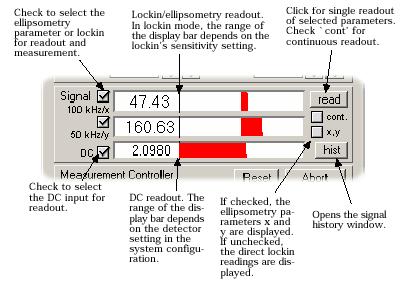
This section provides a readout of the ellipsometry signal. The displays can show lock-in signals or the values of x and y. There is also a readout of the unmodulated detector signal, described as the ‘dc’ signal. Since x and y are calculated from the modulated (or ‘ac’) signal detected by the lock-in amplifiers divided by the dc, the three readouts show all the information that goes into the ellipsometry signal.
If the x,y box is checked, the first two display areas show the x and y ellipsometry signal. If it is unchecked, the displays show the lock-in signal in mV.
The ‘read’ button performs a single readout of the selected signals.
If the ‘cont. read’ box is checked, the signals are updated live (about three times a second). The ellipsometry readout uses the settings specified in the measurement section of the Picometer Ellipsometer Control panel. If the ‘modulate analyser’ option is selected, only single-shot readout should be used, since the analyser modulation takes too long for a continuous live readout. Therefore it is not recommended to use continuous readout mode if both the ‘x,y’ button is checked and ‘modulate pol/ana’ is selected in the measurement section.
When reading the lock-in signal, the range of the upper two bar displays is updated automatically to react to the lock-in sensitivity settings. In ellipsometry mode, the range is fixed to ±1.
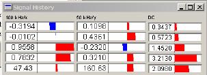
The ‘hist’ button opens a history window that shows the last five signal readouts. The signal values are added to the history in first-in, first-out mode. The history is only updated if the history window is open. This feature is handy for comparing different instrument settings while setting up an experiment.


Measurement Controller Section

There are two buttons in this section:
Reset – this button prepares the controller for taking a measurement by returning the polariser and analyser to 45o and clearing the memory.
Abort – this button stops whatever the controller is doing when it is presses such as moving the arms or taking a measurement.


The Measurement Section

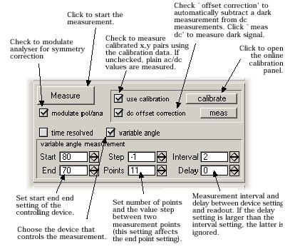
This part of the Picometer Ellipsometer Control panel contains controls for setting the parameters for ellipsometry measurements, and for automatic measurement scans.
An ellipsometry measurement is started by clicking the ‘Measurement’ button. If any of the scan type checkboxes at the bottom of the Measurement Control section are selected, the ‘Measurement’ button starts the scan. Otherwise, the button has the same functionality as the ‘read’ button in the Signal Display section. During a scan this button changes to stop (this stops the data acquisition at that point). Once a measurement is started a Data Display window appears.
The remainder of the measurement section can be split into three parts:

1) Modulation: If the modulate pol/ana box is checked, the polarising element that is selected for modulation is modulated during measurement. This means that two readings are taken at two positions of the polarising element. The readings are subtracted to correct for systematic signal offsets. The two modulation positions are symmetric to the p direction; at the standard polariser/analyser angle of 45o, the second position is 135o. It is recommended to always use this option, unless a fast time response is needed. In this case, systematic offsets should be determined prior to starting the scan.

2) Calibration: The use calibration check box activates the online ellipsometry calibration function of the Measurement Controller. It is recommended to always use the online calibration option, unless the data is to be calibrated with the offline Calibration panel at a later time.
The dc offset correction check box is used to automatically correct for the offset in the dc input channel. The value of the offset must be measured first by clicking the small ‘meas’ button to the right of the checkbox. For this measurement, all light must be blocked from the detector with a black cloth or a similar device. The instrument should be allowed to warm up for at least 30 minutes before measuring the offset (and indeed, before any measurements are taken). It is recommended that the offset correction is always used.


3) Measurement Parameters: At the bottom of the Measurement Control section are the controls for automatic ellipsometry scanning. The scan is started when the ‘Measurement’ button is clicked while any of the scan type checkboxes are checked. If scanning mode is selected, an inset box with the scan parameters appears below the checkboxes. The following options are available:

Time Resolved - Select this to do time scans. The scan parameter box will show fields for the duration, interval, and number of points in the scan. The duration and interval must be given in seconds.

Variable Angle - Select to do angle scans. The scan parameters are the initial and final angle, the angle increment, the number of points, the time interval, and delay. All angles are given in degrees. The initial angle should be larger than the final angle so that the ellipsometer arms drive against gravity. This allows the table drive to position the arms without overstepping during measurement.

Spectroscopic - This is only available if a monochromator is installed. The scan parameters are the initial and final wavelength, the wavelength increment, the number of points, and the time interval, and delay. Two checkboxes allow the wavelength to be specified in nm or as photon energy in eV. The later allows you to run spectroscopic scans with points equidistantly spaced in photon energy.

The ‘interval’ sets the minimum time interval (in seconds) between two measurement points. The ‘delay’ sets the time delay (in seconds) that is applied before the readout is started. If the setting of the device controlling the scan (e. g. Optical Table or monochromator) and the readout of the ellipsometer take longer than the interval time, the interval parameter is ignored. Therefore, in most practical situations the time interval can be set to zero. If the ‘modulate pol/ana’ option is selected for ellipsometry measurements, the readout delay is automatically determined from the lock-in time constant during the two modulation measurements. In this case, which is the default mode of operating the ellipsometer, the delay time should be set to zero. In all other cases, it is important to set the delay time correctly. It should normally be at least six times greater than the lock-in time constant.


Saving Data
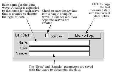
This part of the Picometer Ellipsometer Control panel is used to save measured data into Igor waves. This is similar to saving data in files on the hard disk, except that the data is saved into the current Igor experiment file.
The Igor experiment can then be saved to disk. The individual waves will not appear as separate files on the hard drive, but are part of the Igor experiment. The Igor experiment file is not automatically saved when measured data is copied. Select ‘Save’ from the ‘File’ menu or use the keyboard shortcut ‘Ctrl-S’ to get a permanent copy of your data on the hard disk. To export a data wave into a separate file, use Igor’s data export commands. The last measured data can be copied to either a single complex wave with the x signal in the real part and the y signal in the imaginary part; or as two separate waves for x and y. The wave names are created by appending an underscore character followed by a type code to the text in the ‘Name’ field. The codes are:
ex Real wave with ellipsometry x signal
ey Real wave with ellipsometry y signal
exy Complex wave with ellipsometry x and y signal

The waves are created in the current data folder when the ‘Make a Copy’ button is clicked. The new data waves will appear in Igor’s Data Browser. The ‘User’ and ‘Sample’ fields can be used to enter additional information about the data. This information is stored in the wave note; it can be viewed using the ‘Wave Info’ command in the ‘bi:Data Browser’ menu. Ellipsometry data in Igor waves can be displayed from the data browser with the
Elli Data Graph. It can be used to review both real and complex data.


Ellipsometric Data Graph

The ‘Elli Data Graph’ command in the ‘bi:Data Browser’ menu is a powerful method to display ellipsometry data traces, or one-dimensional ellipsometry waves. Such data is obtained from a measurement scan with the Picometer Ellipsometer, or as a result of a data simulation from the
Multilayer Evaluation panel.
To open a new Elli Data Graph window, first select one or more ellipsometry data waves in the Data Browser. The data must have the same controlling device. For example, you cannot mix a time scan with an angle of incidence scan. However, you can plot as many ellipsometry waves in the same window as you like. Complex waves are automatically expanded to separate x and y, Re(r) and Im(r), or Y and D waves in the display. The data to be displayed may be represented in any of the three common ellipsometry parameters.
The parameter type is identified by the ending of the wave name: Standard x, y data - ex, ey (real); exy (complex), Re(r) and Im(r) data - er, ei (real); eri (complex) and Y and D data - ep, ed (real); epd (complex). In the list above, the first two types of endings represent data of a single parameter in a real valued wave, and the last type of ending denotes a complex wave with the first parameter in the real part, and the second in the imaginary part. The standard format used by Beaglehole Instruments is the x, y format.

The toolbar at the top of the window has four buttons in it:
r - Click to restore the display area to show all data, that is, to autoscale all axes. Use this to restore the graph after zooming around in with the marquee.
i - Show or hide the info area at the bottom of the graph. It has two cursors that can be dragged onto a trace in the graph. Information about the data values and the value difference between the two cursor positions are shown in the info area. If the window is too small to display all the available information, use the small scroll areas to scroll the info display.
l - Show or hide the legend. The legend can also be dragged with the mouse. Cycle through the three axis modes:
Left axis only: All traces are plotted against the left axis.
Left/right axis: x/Re(r)/Y traces are plotted against the left axis, and y/Im(r)/D traces are plotted against the right axis. This is usually the most convenient mode because the autoscaling of the axes works better in this mode if x and y data are very different from each other.
y/Im(r)/D vs x/Re(r)/Y: Plotting one parameter against the other is often used to analyse ellipsometry data. In this mode, each pair of waves with the same base name results in a single trace in the display.

The ellipsometry parameter popup menu allows the choice of three different ellipsometry parameters to be used for displaying the data:
x, y - the standard phase modulated ellipsometry parameters.
Re(r), Im(r) - the real and imaginary part of the complex reflectivity ratio r = rp/rs.
Y and D - the traditional rotating element ellipsometry parameters. These are also related to r through the relation r = tanY exp(iD). (If these parameters are selected, a checkbox appears to the right of the popup menu, offering the choice to limit the values of Y and D to below 180o. This is the format used by most rotating element ellipsometers and other optical simulation software.)
The data is converted to the other parameters for display only, leaving the original data in x, y format. If the original data is changed, its trace in the Elli Data Graph also changes accordingly.

If the ‘Alt’ key is pressed and held while clicking inside the display area, the portion of the graph that is displayed can be moved around the display area. This is a convenient way of scrolling around a zoomed display. To zoom in or out, click on any empty part of the display area and drag open a marquee. The marquee has handles that can be used to resize it. It can be moved around by grabbing the marquee frame with the mouse. Clicking inside the marquee opens a context menu with options to expand or shrink the displayed portion of the graph. To restore the axes so that all data is shown, click the ‘r’ button in the toolbar. A trace in the display can be offset by clicking on it and holding the mouse button down for a few seconds. The trace can then be moved around with the mouse. Holding the ‘Shift’ key while moving a trace restricts the movement to one dimension. As with all graph window functions, the original data is not affected by this.

Igor’s standard graph window commands can be used to manipulate Elli Data Graphs. However, some types of changes are lost when changing the axis mode. For instance, annotations are retained, but axis labels are lost. When an Elli Graph Window is closed, there is no dialog for saving a recreation macro. Elli Data graphs cannot be saved to a macro.
Elli Data Graphs can be included in Igor layout windows. The toolbar will not show in a layout. Use ‘Windows:New Layout. . . ’ to create a new layout. Layouts are used to arrange one or more graphs on a page for printing. Elli Graphs can also be embedded in Igor notebooks. This can be used to write reports directly in Igor.


Data Display

Once a measurement is started a Data Display window appears. This window is similar to the
Elli Data Graph, with a few exceptions:
The data is always displayed in the x and y parameters. There is no parameter popup menu.
There is an additional ‘z’ option in the toolbar which can be used to zero the display, that is, to erase all data from it.
The window has a grey background, which is not very convenient for printing. Copy the measured data and use an Elli Data Graph instead.
The window only displays the last measurement data.

The toolbar buttons (except for the ‘z’ button which is described in the list above) and the marquee work exactly as they do in an Elli Data Graph window.


Data Analysis

Once the ellipsometry data has been acquired it is necessary to model it to extract physical parameters of the sample. Generally this is the hardest part of the experiment and below is only given the minimum explanation of the options open to you. For more advice information contact the
Surface Analysis Facility.

Single wavelength ellipsometry data can be modeled using Beaglehole instruments Multilayer Evaluation Panel accessed through the bi menu. This simulates data either with layer thickness or angle of incidence for a defined layer stack. When a simulation is produced the waves created are displayed in the Multilayer Evaluation data display which has some of the display options of a Elli Data Graph window.

Spectroscopic Data can be modeled using SCI Film Wizard. For this the waves must be exported as a “Target” file using ‘Export As Film Wizard Target’ option in the ‘bi:Data Browser’ menu. This takes an x,y pair of data and creates a Target file that can be read by Film Wizard. To export data, select a pair of x and y data waves or a single complex ellipsometry data wave in the data browser, and then select ‘Export As Film Wizard Target’. If the export routine cannot find all the information that is needed to export the data in the waves themselves, a dialog box prompts you for any missing parameters. Finally, a standard file save dialog appears that allows the user to choose a destination for the Target file, the file save dialog will automatically change into Film Wizard’s ‘Target’ directory so that the file can be located immediately from the Target window in Film Wizard. Currently, Film Wizard’s calculation routines only support the traditional ellipsometry parameters Y and D.


Back to the instruments page